Predict Plot for adjusted Gamlss model

Following the example of book "Flexible Regression and Smoothing Using GAMLSS in R", the plot of the predicted values, adjusted, can be done following the example below.

library(gamlss)
library(dplyr)
library(ggplot2)
data(film90)

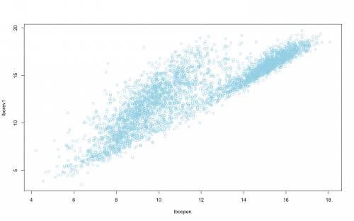
# plot das observacoes
plot(lborev1~lboopen, data = film90, col = "lightblue")

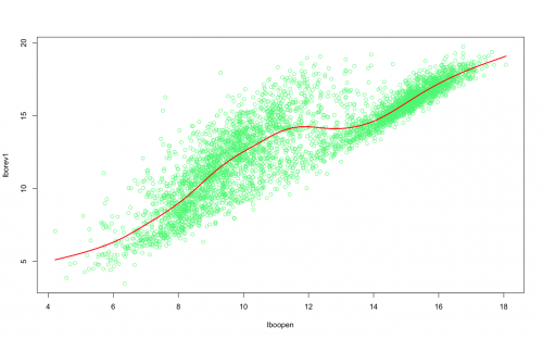
model <- gamlss(lborev1~pb(lboopen), data = film90, family = NO)

# plot das observacoes + valores ajustados
plot(lborev1~lboopen, col = "lightgreen", data = film90)
lines(fitted(model)[order(film90$lboopen)]~
        film90$lboopen[order(film90$lboopen)], col = "red", lwd = 2)

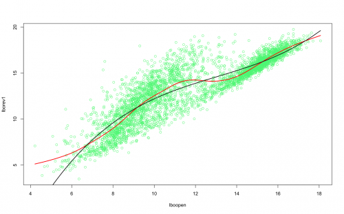
film90 <- film90 %>% 
  dplyr::mutate(lb2 = lboopen^2,
                lb3 = lboopen^3)
model2 <- gamlss(lborev1~lboopen + lb2 + lb3, data=film90, family=NO)

plot(lborev1~lboopen, col = "lightgreen", data = film90)
lines(fitted(model2)[order(film90$lboopen)]~
        film90$lboopen[order(film90$lboopen)], col = "grey10", lwd = 2)

{
  plot(lborev1~lboopen, col = "lightgreen", data = film90)
  lines(fitted(model)[order(film90$lboopen)]~
          film90$lboopen[order(film90$lboopen)], col = "red", lwd = 2)
  lines(fitted(model2)[order(film90$lboopen)]~
          film90$lboopen[order(film90$lboopen)], col = "grey10", lwd = 2)
}

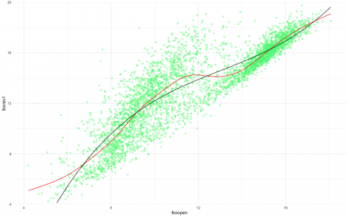
You can also plot using ggplot2.

ggplot2::ggplot(film90) +
  geom_point(aes(x = lboopen, y = lborev1), col = "lightgreen", alpha = 0.5) +
  geom_line(aes(x = film90$lboopen[order(film90$lboopen)],
                y = fitted(model)[order(film90$lboopen)]), col = "red") +
  geom_line(aes(x = film90$lboopen[order(film90$lboopen)],
                y = fitted(model2)[order(film90$lboopen)]), col = "black") +
  scale_y_continuous(limits = c(4, 20),
                     expand = c(0, 0)) +
  theme_minimal()

Since your example is not fully reproducible, I adapted a little this one from the book. But I believe that you will have no problem adapting to your case.

term.plot(model2, pages = 1, partial = T)

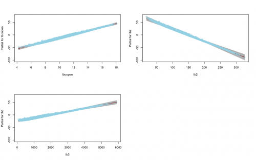
Larger examples of term.plot() use can be found here or here..